VisualCaseGen: Fill Indian Ocean with land

!!! This page is under construction !!!

These instructions describe how to modify the continental geometry in an uncoupled case using the VisualCaseGen tool.  In the example given, the Indian Ocean is filled in with land and the new land regions are specified as c4-grass.  Instructions are provided here for the same example but using the fsurdat and mesh mask modifier tools from the command line.  

Step 1: Install and launch VisualCaseGen and select "Custom" case.

Download and install the VisualCaseGen tool following the instructions here.  Once you have launched VisualCaseGen and executed the first cell you should see something like this:

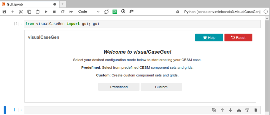
Here, we are not running a basic predefined case with CESM.  We are modifying the configuration substantially by changing the continental geometry, so you should select "Custom" here. 

Step 2: Select the model components.

Having selected custom mode, you should now see a cell like the one below that allows you to select the time period of simulation (1850's forcings, 2000's forcings, transient historical) as well as the different model components to use and any special options within those components.

Here, we will select to run a 2000 case by clicking on the "2000" button.  Then we select the following component options: cam as the atmosphere; clm as the land component; cice as the ice component (this is necessary even in a prescribed sea ice simulation because while the ice fraction is prescribed and the ice thickness is relaxed toward 2m in the Northern Hemisphere and 1m in the Southern Hemisphere, the 1d thermodynamics of the sea ice model is still being used to compute surface fluxes, snow depth, albedo and surface temperature over the ice); docn (or data-ocean) which indicates that we will use prescribed SST; rtm as the river transport model; sglc (or "stub" land ice) which indicates that the land ice model will not be active; and, swav (or "stub" wave model) which indicates that the wave model is not active.  In general, the "s"component options indicate "stub" component options that are not active, and the "d"component options indicate data components where the fields of importance are being prescribed.  

As you choose options, VisualCaseGen will cross out options that are incompatible with your choices.  In the end, our choices for this case look like this:

 The "Physics and Options" tabs below this allow you to specify the physics and other options for your case.  For CAM we'll select CAM6 physics

For CLM, we'll choose CLM5 and "satellite phenology" mode, which means that aspects of the land model such as leaf-area index are prescribed in the model as opposed to being prognosed interactively by the biogeochemistry aspects of the land model.

For the sea ice component, we now have to select that we will use "prescribed ice" from the physics and options tab

For the ocean component, the prescribed ocean mode is already selected

for the river, land ice and wave components, we have no modifiers to select.

Step 3: Select the model grid

After you have selected your model components, you'll see a section where you can select your model grid. This can either be a "predefined" grid i.e., a grid that's already available and used within CESM, or it can be a "Custom" grid. While, in this case, we are going to use a standard resolution, we are going to change the grid in terms of the areas that are land versus ocean. So we will select the "Custom" option here.  When you select "Custom" you'll see tabs that allow you to make selections regarding the atmosphere and land grids.

For the atmosphere, the VisualCaseGen tool expects you to choose an existing atmosphere grid within CESM.  Here, we'll choose the standard 1 degree resolution "0.9x1.25"

Now we move to the "CLM Grid" tab and this is where all the modifications will be performed to fill in the Indian ocean with land.  First we need to select a base land grid.  Since we're using the standard 1 degree resolution in the atmosphere, we'll select that for the land as well

Step 4: Modify the mesh file

When setting up a coupled case, the ocean component determines the land mask.  Here, we are setting up an uncoupled case, so we need to use the mesh mask modifier tool here to set up the mesh file to contain the correct land mask.  You can find out more about mesh files here.  You should see something close to the screenshot below where you can now select the inputs to the mesh mask modifier tool.  

The VisualCaseGen tool has already selected the default input mask mesh for the 0.9x1.25 grid.  Now we are going to modify that by giving the tool a netcdf file that contains our chosen land mask in the "Land mask (pre-generated by user)" section.  This netcdf file should contain the following variables.

landmask(lsmlat,lsmlon)	landmask containing 1's for land, 0's elsewhere
mod_lnd_props(lsmlat,lsmlon)	mask where the surface properties will be altered (1's for modification, 0's elsewhere)
lats(lsmlat)	the latitudes of the grid
lons(lsmlon)	the longitude of the grid

You can call the longitude and latitude dimensions and variables anything you like, you just need to provide VisualCaseGen with those names in the "Latitude Var. name", "Longitude Var. name", "Latitude dim. name" and "Longitude dim. name" boxes in the screenshot above.

In this example, where the default continental geometry is being modified, you can first find the default landmask and modify that (see the instructions for finding the default land mask here).  This example script uses the default landmask for an FHIST case in CESM2 at 0.9x1.25 resolution (the f09_f09_mg17 grid) and produces the mask required for the fsurdat modifier tool as depicted in Figure 1.

Let's call the file that contains these new masks "mask_fillIO.nc" and suppose we have placed it in the folder /glade/u/home/islas/python/CSSI/modifylandmask_scripts/.  We will now select that file from the menu.  Since we have also called the longitude and latitude variables "lons" and "lats" instead of "lsmlon" and "lsmlat" we'll have to change that too.  We'll also need to select a location for the output mesh mask file.  We'll put this in /glade/u/home/islas/python/CSSI/fillIO_files/fillIO_mesh_mask.nc

Now you can run the mesh mask modifier tool by clicking the green button.  This can take some time. 

Step 5: Modify the land surface dataset

Now that we have created our mesh file which determines which grid points are land, we need to modify our land surface dataset.  This is the next stage in the VisualCaseGen tool

The "fsurdat" file controls the land surface properties and their time evolution (where relevant).  You can read more about fsurdat files here.  VisualCaseGen has already found the default surface dataset for a year 2000 simulation using satellite phenology mode at this resolution and selected it as the "Input Surface Dataset".  We are going to specify the land points where we want to modify the land surface properties using mask input from a file (recall the mod_lnd_props mask we generated in Step 3).  So we'll select "via mask file" and since we have already used a file to specify the land mask, it has selected this same file by default.  If you would like to see the area you are modifying you can also click the "preview" button and it will show a map illustrating the area you're changing (with value = 1).

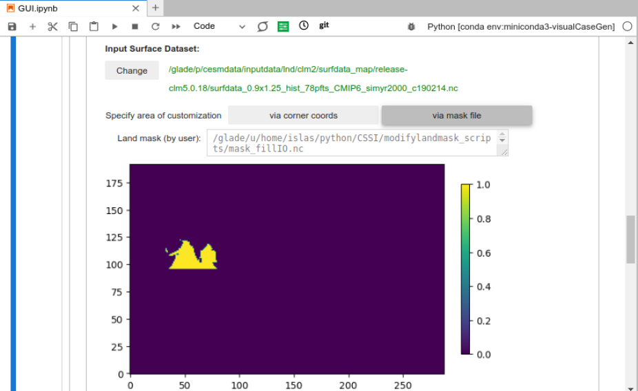
If your modification to the land surface properties are simpler, you could instead choose the corner coordinates of the region you'd like to modify by specifying the "via corner coords" option for "Specify Area of Customization".

Below this, you'll see various options that you can select for your land surface data type.  We'll choose the "Idealized" option which allows us to specify our idealized land surface properties where mod_lnd_props=1.  We then select our plant functional type (PFT) to be 14 which corresponds to c4-grass in this case.  The PFT numbers and names may change depending on which model version or configuration you're using, but you can look in the "paramfile" for the default case to find out the numbers that correspond to different PFTs for your case (see section 2.2 here).  We'll also set the soil color to 10, the standard deviation of elevation to 0, the max fraction of saturated area to 0, leaf area index to 3, the stem area index to 1, the top height of the canopy to 1 m and the bottom height of the canopy to 0.5 m for each month of the year.  Finally, we will specify the output file for this surface dataset as /glade/u/home/islas/python/CSSI/fillIO_files/fillIO_fsurdat.nc.

Now you can run the fsurdat_modifier tool but pressing the green button.  This can also take some time.  Once it has finished, you should see the fsurdat file has been created at the location you gave for the "Output Surface Dataset". 

Step 6: Create and configure the case

The final step is to create your case and configur it to use your new mesh and fsurdat files.  You have two options.  The final "Launch" section of the GUI helps you to do this.  

 There are two options here.  (1) You can get the GUI to create the new case for you by pressing the green "Create new case" button or (2) You can get the GUI to show you the commands required to create and configure the case.

First you can the path you would like the case to be create at using the "Select" button.  In this example, we will build create the case at /glade/scratch/islas/f.e23_f09_f09_fillIO.001.  If you are running on the NCAR supercomputers you will also need to put your Project ID into the Project ID box.

If you select the green "Create new case" button, it will create and configure the case for you.  Alternatively, if you select the blue "Show commands" button, it will tell you the commands required to create and configure this configuration.  For the above case, the output from the "Show commands button" looks like this

 

This is the option you would want to use if you plan to run this case from a different tag or on a different machine from where you have run VisualCaseGen.  These commands are telling you how to do the following things

• Set up the case with the required compset at your chosen using the "create_newcase" command on your chosen machine.
• Change into the case directory !!! still to do !!!
• Run the xmlchange command to set up your atmosphere grid
• Run the xmlchange command to specify the mesh file !!! seems incorrect !!!
• Information on how to point to your new fsurdat file !!! this isn't there !!!
• Create the case

Now you have configured your case with the Indian Ocean filled with land and you should be able to build and run it in the same way as other CESM cases.