VisualCaseGen: Ridge World

!!! This page is under construction !!!

This example provides step-by-step guidance on how to generate a coupled idealized configuration that consists of an aquaplanet with land caps at the pole and a narrow land ridge extending between the two poles, similar to the configuration used in Wu et al (2021).  In the example given below, the visualCaseGen GUI is used to guide users through choosing their CESM components, setting up all the ocean input files, setting up all the land input files, and finally setting up and configuring their case.

Step 1: Install and launch VisualCaseGen and select "Custom" case

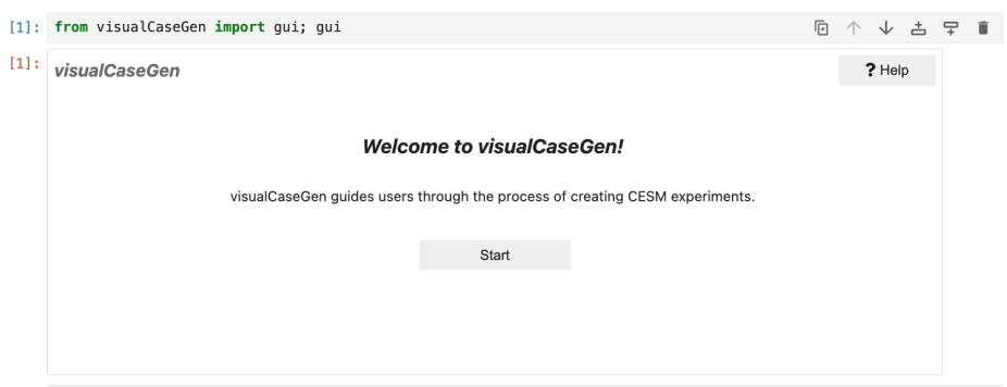
Download and install the VisualCaseGen tool following the instructions here.  Once you have launched VisualCaseGen and executed the first cell you should see something like this

Click on the start button and then you should see something like this

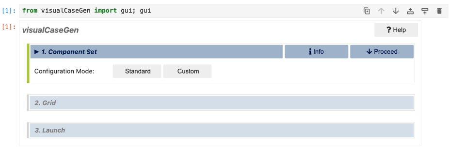
Here we are not running a standard case with CESM.  We are modifying the configuration substantially by changing the ocean grid, ocean bathymetry, continental geometry and land surface properties, so you should select "Custom" here.

Step 2: Select model components

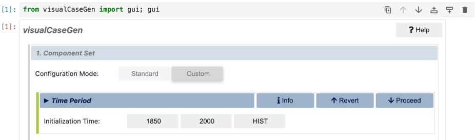
Having selected custom mode, you should now see a cell like the one below that allows you to select the time period of simulation (1850's forcing, 2000's forcing, transient historical).  Here we will select to run an 1850 case by clicking on the "1850 button"

Once the 1850 time period has been selected, the option to choose individual model components will become available like this

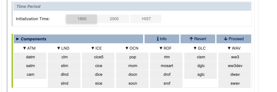
Here you can select the individual model components you'd like to use and then the following cell allows you to select specific options for those components.   In this ridge world case we select the following component options: cam as the atmosphere; clm as the land component; cice as the ice component; mom as the ocean component, srof (i.e., stub run off) as the river component; sglc (i.e., stub land ice) as the land ice component; and, swav (i.e. stub wave) as the wave component.  In general, the "s" component options indicate "stub" components that are not active.

As you choose options, VisualCaseGen will cross out options that are incompatible with your choices.  In the end, our choices for this case look like this and the cell below now becomes available to make specific choices within each component:

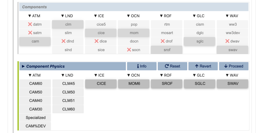
The "component physics" cell allow you to specify the physics within each component for your case.  In this case it's only the atmosphere and land components that have multiple choices.  Since we're following the setup of Wu et al (2021) we'll choose CAM4 as the CAM physics option and CLM5 as the land option.  Once selected, the component options cell will be triggered below which allows you to select specialized options for each component.

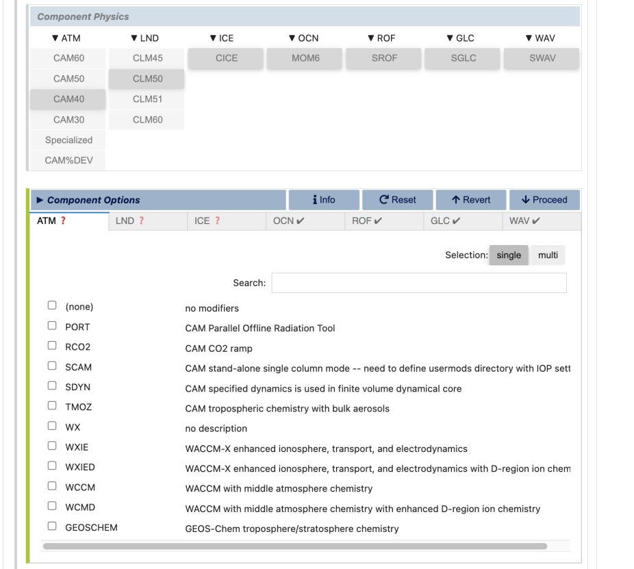
For the atmosphere, we won't select any modifiers by slecting "none".  Then clicking on the LND tab will open up the choice of modifiers for the land model.  Here we'll select the satellite phenology (SP) mode for the land which means that aspects of the land model such as leaf-area index are prescribed as opposed to being prognosed interactively by the land biogeochemistry.

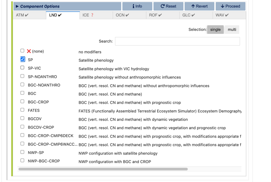
For the ice we'll also select no modifiers by clicking "none" and for the other components there are no other options to select from.

Step 3: Select the model grid

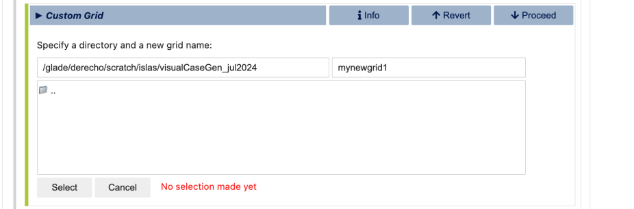
After you have selected your model components, you'll see a section where you can select the model grid.  This can either be a "Standard" grid i.e., a grid that's already available and used within CESM, or it can be a "Custom" grid.  Here we are defining our own ocean grid and we're going to change the bathymetry and land mask, so we need to select the "Custom" option.  When you select "Custom" you'll be given the option to specify a directory and a name for your new grid.  The directory is where all the new grid files will be stored and the name will be the name that will be used to refer to this new grid for the rest of the configuration process and in your CESM simulation.  

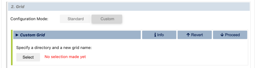
Upon clicking the "Select" button, you'll be given the option to enter a directory path and a name for your new grid.  Note that you will need to make sure this directory already exists so that you can select it.

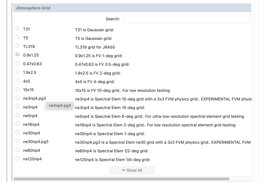
Once you have chosen your grid directory and name and clicked "Select", you'll be given the option to specify the atmosphere grid.  For the atmosphere, you are expected to choose an existing atmosphere grid within CESM.  Here, we'll choose the standard 1 degree resolution"0.9x1.25"

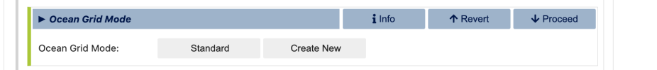
For the ocean, we're going to create our own new ocean grid as opposed to using a standard grid.  So, in the next cell click "Create New"

This will open up the option to select whether your ocean is zonally reentrant or not as well as to specify the resolution in the zonal (x) and meridional (y) directions.  Note that CAM cannot run in a regional configuration, so since we have selected CAM4 as our atmospheric component, the "Regional" grid extent option is not available to us and the ocean has to be "Zonally Reentrant".

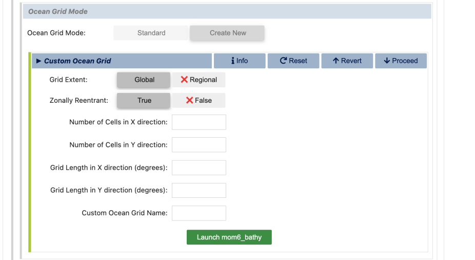
We'll specify 360 cells in the x direction and 180 cells in the y direction and specify the length of the grid in the x direction to be 360 degrees and the length of the grid in the y direction to be 180 degrees.  Note that the grid length expected here is the total length across all grid cells as opposed to the length of an individual grid cell.  You'll also have to give your custom ocean grid a name 

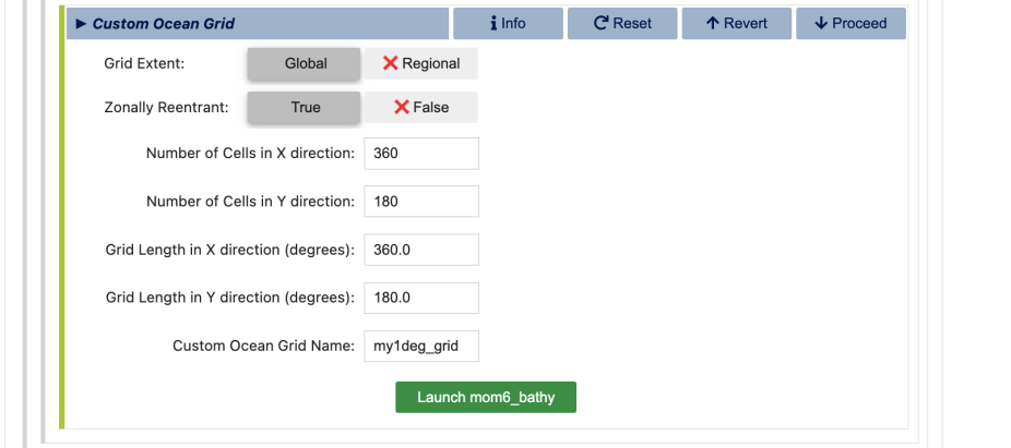
Once all slections have been entered we can press the green "Launch mom6_bathy" button.  This will launch the mom6_bathy tool that in a separate jupyter window and this can be used to set up the ocean bathymetry, land mask, and associated ocean model input files.  Upon launching the mom6_bathy tool, it will likely ask you to select a python kernel.  Make sure to select the VisualCaseGen environment.

Step 4: Configure the ocean bathymetry

Once the mom6_bathy tool has been launched by VisualCaseGen, you should see a jupyter notebook that looks something like this

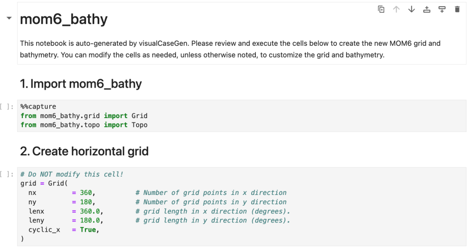
The first two cells here have already been populated automatically by the visualCaseGen tool.  You can see in the "Create horizontal grid" cell that our choices for the grid resolution have already been populated there e.g., we have 360 grid cells in the longitude direction and 180 grid cells in the latitude direction along with total grid lengths of 360 degrees in the longitude direction and 180 degrees in the latitude direction and a zonally reentrant ocean since cyclic_x = True.

Execute these first two cells to update the MOM6 supergrid.

The third section of mom6_bathy can be used to set up the bathymetry.  The default options are to produce an ocean of depth 2000m with a minimum depth of 10m but we are going to instead generate an ocean that resembles the ridge world case of Wu et al (2020) which has a depth 4000m with some sinusoidal fluctuations at the surface, a land ridge of width 1 degree longitude and the furthest poleward 10 degrees latitude at the poles set to land.  There are three different ways in which you can achieve this: (1) specifying this analytically with python code within mom6_bathy; (2) reading this ocean set up in from a file; or (3) using the point and click feature of the mom6_bathy tool.  We now outline how to use each of these different methods.

Option 1: Specify the bathymetry using python formulae

Within the section of mom6_bathy called "3. Configure bathymetry" you can first instantiate the "topo" object and then modify the depth of the bathymetry as outlined below.  Make sure to remove the code that already exists within this section other than what you want, so that it should end up looking something like this

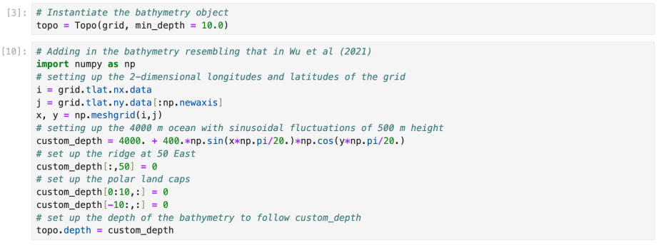
In this code we have set up the 4000 m deep option, with sinusoidal fluctuations and set the depth of the ocean to 0 at all latitudes at 50 degrees east and at all longitudes over the 10 degrees latitude range at the poles.  You will need to execute these cells and then you can plot the bathymetry to check it looks like what you were expecting:

 

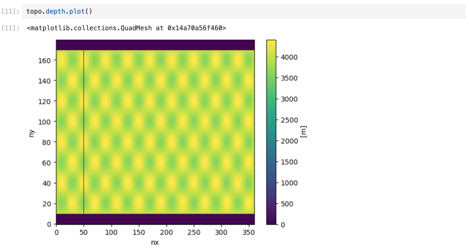
Here we have a very narrow (1 degree wide) land ridge at 50 degrees and polar land caps with sinusoidal fluctuations along the 4000 m deep ocean floor.

Option 2: Read in your bathymetry from a file

!!! coming soon !!!

Option 3: Use the point-and-click bathymetry selection option in mom6_bathy

!!! coming soon !!!

Step 5: Save the ocean bathymetry files

The final section of mom6_bathy (4. Save the grid, bathymetry, and mesh files) can be executed to save the MOM6 supergrid file, the MOM6 bathymetry file, the CICE grid file and the ESMF mesh file.  By default, this saves the files into a subdirectory within the directory you specified in step 3 and the name of that directory is the name you gave to the ocean grid also in step 3:

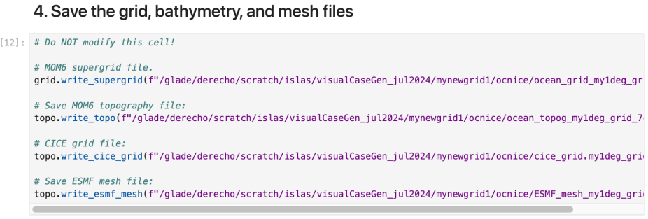
If this cell executes successfully then you should see four files have been created in the location you specified.  Now you can return to the VisualCaseGen GUI to configure the land surface.

Step 6: Configure the land surface properties

Return back to the VisualCaseGen GUI and proceed to the Land Grid Mode

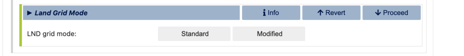
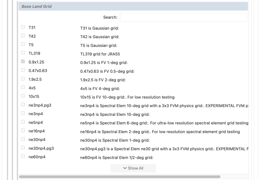
Here we'll also be using a modified land grid since we have idealized continental geometry.  So click "Modified".  The first step in defining the land grid is to choose the base land grid from a selection of default CLM grids.  Since we chose the standard 1 degree resolution in the atmosphere, we'll select that for the land as well i.e., the option "0.9x1.25".  

Based on this choice VisualCaseGen will now populate the "Input surface data file (fsurdat)" with the appropriate file e.g.,

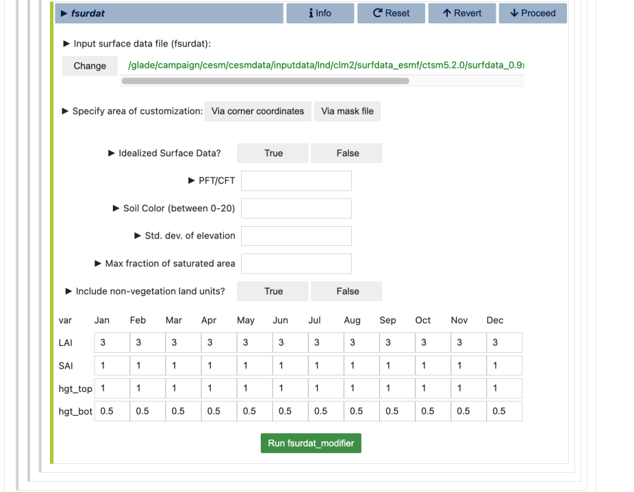
The "fsurdat" file controls the land surface properties and their time evolution (where relevant).  You can read more about fsurdat files here.  The remainder of this section of VisualCaseGen can be used to specify the land surface properties over our idealized land regions.  Since we are modifying the whole planet, we can specify the region to modify using the "via corner coords" and modify from 90 degrees South to 90 degrees North over longitudes from 0 degrees to 360 degrees.  We'll also use the "Idealized" option.  

We need to set the land surface properties by specifying the plant functional type (PFT).  The PFT numbers and names may change depending on which model version or configuration you're using, but you can look at the "paramfile" for a default case using your resolution and forcing period to find out the numbers that correspond to different PFTs for your case (See section 2.2 here).  We'll use the PFT of zero which for this case corresponds to bare ground.  Note that Wu et al (2021) actually specified the land surface to  be wetland but this option is not yet available within VisualCaseGen.  

We'll also specify the soil color to be 10, the standard deviation of elevation to be zero and the max fraction of saturated are to be zero.  We will keep "Include non-vegetation land" as True since we want to set the surface to bare ground in this case.  You can leave the specification of leaf area index, stem area index, canopy top and bottom as the defaults because this will have no effect in a case where we are setting all the land to be bare ground without vegetation.  After making these choices, this part of the GUI should look something like this  

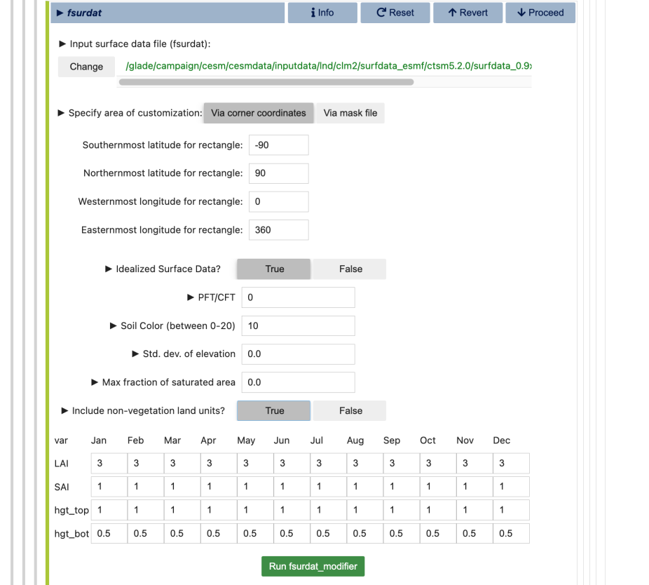
Now click on "Run fsurfat_modifier" to generate the fsurdat file.  This can take some time.  Once it has completed it will produce the fsurdat file within a subdirectory of the directory you specified in step 3.

Step 7: Set up and configure the case

The final step is to create your case and to configure it to use your new ocean files and fsurdat files.  You have two options for doing this through the final "Launch" section of the GUI.  

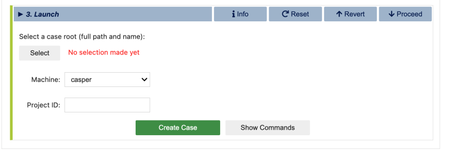
If you have run VisualCaseGen from within the CESM tag and on the machine that you would like to use to run the simulation then you can simply specify the case path in the "Select New Case Path" section and VisualCaseGen will run create_newcase and all the commands to configure the case to use your new MOM6 files and fsurdat file.  Otherwise, you can click on the "Show commands" button to see the commands you would need to execute to set up this case using the tag that you would like on the machine you would like.  You'll still need to select the case path if you're using the "Show commands" option.

If you press the show commands button you'll see the following:

Creating case...

• Updating ccs_config/modelgrid_aliases_nuopc.xml file to include the new resolution "mynewgrid1" consisting of the following component grids.
 atm grid: "0.9x1.25", lnd grid: "0.9x1.25", ocn grid: "my1deg_grid".

• Updating ccs_config/component_grids_nuopc.xml file to include newly generated ocean grid "my1deg_grid" with the following properties:
 nx: 360, ny: 180. ocean mesh: /glade/derecho/scratch/islas/visualCaseGen_jul2024/mynewgrid1/ocnice/ESMF_mesh_my1deg_grid_7c8432.nc.

Running the create_newcase tool with the following command:

/glade/work/islas/cesm2_3_beta17_gui/cime/scripts/create_newcase --compset 1850_CAM40_CLM50%SP_CICE_MOM6_SROF_SGLC_SWAV --res mynewgrid1 --case /glade/derecho/scratch/islas/visualcasegen_case.001 --machine derecho --run-unsupported --project P04010022 --non-local 

Navigating to the case directory:

cd /glade/derecho/scratch/islas/visualcasegen_case.001

Running the case.setup script with the following command:

./case.setup --non-local

Adding parameter changes to user_nl_mom:

  INPUTDIR = /glade/derecho/scratch/islas/visualCaseGen_jul2024/mynewgrid1/ocnice
  TRIPOLAR_N = False
  REENTRANT_X = True
  REENTRANT_Y = False
  NIGLOBAL = 360
  NJGLOBAL = 180
  GRID_CONFIG = mosaic
  TOPO_CONFIG = file
  MAXIMUM_DEPTH = 4400.0
  MINIMUM_DEPTH = 10.0
  DT = 900
  NK = 20
  COORD_CONFIG = none
  REGRIDDING_COORDINATE_MODE = Z*
  ALE_COORDINATE_CONFIG = UNIFORM
  TS_CONFIG = fit
  T_REF = 5.0
  FIT_SALINITY = True
  GRID_FILE = ocean_grid_my1deg_grid_7c8432.nc
  TOPO_FILE = ocean_topog_my1deg_grid_7c8432.nc

Adding parameter changes to user_nl_cice:

  grid_format = "nc"
  grid_file = "/glade/derecho/scratch/islas/visualCaseGen_jul2024/mynewgrid1/ocnice/cice_grid.my1deg_grid_7c8432.nc"
  kmt_file = "/glade/derecho/scratch/islas/visualCaseGen_jul2024/mynewgrid1/ocnice/cice_grid.my1deg_grid_7c8432.nc"

Adding parameter changes to user_nl_clm:

  fsurdat = "/glade/derecho/scratch/islas/visualCaseGen_jul2024/mynewgrid1/lnd/0.9x1.25_fsurdat_modifier.nc"

• Set up the case using the create_newcase command
• Change directories into your case directory to configure the case !!! this isn't there !!!
• Run the xml commands to tell the case about your new mesh files for the various components and the configuration of the ocean grid
• Set up the case.
• Once you have set up the case, the namelist files for each component will be produced in your case directory.
• You then need to add the namelist parameters into user_nl_mom and user_nl_cice as described above.